Denis Bakin
Stereoscopy on Complex Scenes and Edge Detection
Contents
Conventional Edge Detection Techniques
The goal of the edge detection is to find discontinuities in photometric and geometric properties of physical objects represented by a 2D image [1]. Although the discontinuities in the photometric properties of the objects are quite important for many applications the geometric shape of the objects is of much more interest, especially for the object recognition. Unlike a conventional 2D picture that does not carry the information about the third dimension, a stereoscopic image encodes the information and can be used to recover at least some of it. The stereoscopy is a method of using binocular (stereoscopic) images, in other words images of the same scene taken from 2 "shifted" positions, to reconstruct a 3D scene. The reconstructed third dimension data can be used for various purposes including detection of the edges representing only the discontinuities in the geometric properties of the pictured objects.
The goal of this work is to try to create an algorithm capable of recovering the depth map of a complex scene represented by a calibrated stereoscopic image, and to do it with a quality good enough for consequent use of the map recovered with conventional edge detection techniques for determining only the discontinuities in the geometric properties of the scene objects.
A successful detection of the geometric edges would allow to reach high levels of abstraction, improve reliability of the objects recognition and can be used for the real objects contour maps generation.
The work slightly touches several huge areas of the computer graphics. The edge detection, image segmentation and stereoscopy techniques are in the focus of the interest here. Below one can find a short overview of the techniques.
Conventional Edge Detection Techniques
Edges:
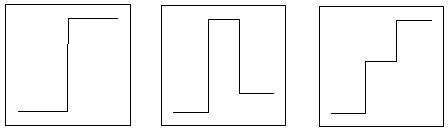
Edges pictured by a 2D image can be classified into 3 basic types (based on the color intensity change)[1]:
Ideal edge, pulse edge and staircase edge.
A three steps process lays in the foundation of great majority of contemporary edge detection systems. These steps are: differentiation, smoothing and labeling.
Differentiation:
At the differentiation step an edge detector calculates gradient of the color
intensity over the image plane and its direction:
The second order derivatives may also be calculated and used instead of the
gradient for the edge detection.
Smoothing:
In order to reduce the false detection caused by noise the image data must be
filtered. The filtering is done by convolving the analyzed data with a filtering
function. The common examples of the filtering functions are Green and
Gaussian functions:
The parameters d
and m
here are usually called scale and
determine the degree of smoothing. The correct choice of the scale is the
major problem of the edge detection. The too high value can cause data loss, the
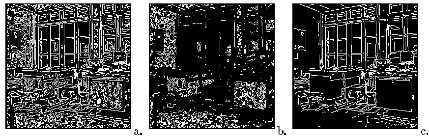
too small value can leave too many edges caused by noise. See examples from [1]:
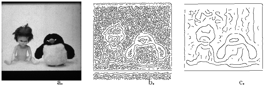
(a) Original image, (b) Gradient maxima detected at scale d=1, (c) Gradient maxima detected at scale d=4
Labeling:
The edge labeling involves
localizing edges and increasing the signal to noise ratio by suppressing the false
edges [1]. An example of the labeling methods for a gradient magnitude
based detector would be the non-maximum suppression (finding local maximums of
the gradient magnitude by measuring along the gradient direction). A thresholding algorithm (for
example hysteresis algorithm: gradient maxima for all edge
points is above the low threshold and at least one point is above the high
threshold) may also be used to filter even more of the false edges. The second order derivative based edge detection
methods use slightly different but not less efficient methods. Example of a
degree of the noise reduction at the labeling stage from [1] are below:
(a) All edges detected at d=1, (b) Noise edges only, (c) Noise edges suppressed
The recent improvements of the edge detection algorithms mostly involve the labeling stage. A method described in [2] explains a technique improving edge detection of the gradient based systems by computing the ideal edge template, comparing it to the real data and using the comparison result as an additional to the gradient magnitude criteria for the edge detection.
The goal of the image segmentation is to separate an image into homogeneous regions. There is a number of image segmentation techniques. Two of the most popular of them are the watershed and the mean shift based methods. There also are lots of various other techniques, for example based on use of the Voronoi diagrams or Markov chains properties. There is no the best for all technique. The desired application of the image segmentation technique determines its suitability.
Watershed
The watershed technique is one of
the most successful image segmentation techniques. In order to grasp intuitively
the idea of the
method, imagine a grey color image as a topographic plane, place sources of
color water (markers) in the largest lows of the plain and start filling the
plain with the water. When the water of the different colors collide, erect a dam at the point
of the collision. Finally all the plain will be filled in with water and
the dams built will separate the final segments. An example of the watershed
technique applied to a 1D function separating it into four regions is presented
below (from [7]):
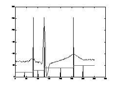
Note that the region boundaries here are at the three maximums of the function.
When applying the watershed algorithm, the most difficult task is the initial selection
of the
markers.
Mean Shift
The mean shift image segmentation
is well described in a relatively small number words in [2]. The idea of the method is to
map all pixels of a picture to a 5D space (for color pictures), where three dimensions represent the
color space and the other two the conventional x,y coordinates.
Then, for each pixel x calculate the average of the |[x]-xi|
where the xi
represents all the neighbors of x
in the distance h
(in the 5D space), thus given a mean shift for the pixel x.
The process is repeated again and again for all pixels after the pixels are virtually
moved along the mean shift gradient vectors. Eventually, the new virtual positions for all
the
pixels of the picture converge and the pixels can be separated into clusters, which are
then recursively fused and form
the final regions.
The improvement of the technique proposed in [2] involves the use of the edge detection to guide the mean shift calculation and the region fusion of the conventional mean shift algorithm explained above. The examples (from [2]) of running the traditional and the improved mean shift segmentation algorithms are below.
(a) - the original image; (b) - the improved mean shift segmentation; (c) - the traditional mean shift segmentation;
3D reconstruction
A stereoscopy assumes availability
of 2 images picturing the same scene from 2 slightly shifted positions:
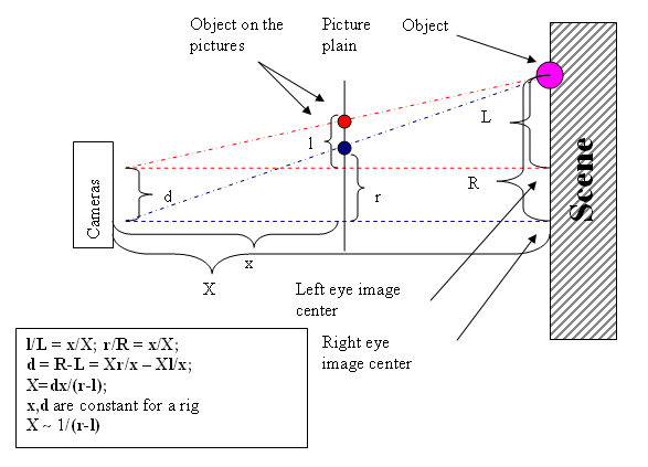
The diagram above (a view from top) represents a simplified case (distance change caused by height is not accounted for) - a stereoscopy rig of two cameras picturing a scene. Basically the only information needed for a reconstruction of a 3D scene at the scale 1/dx is the distance between correspondent pixels on the left and right eye pictures.
Methods
All the stereoscopy calculation methods can be classified into active and passive. The active methods employ various means for marking a position on the scene in order to be able to undoubtedly identify it on the pictures. The passive methods rely only on the natural variances for the matching areas identification.
A straightforward method of computer based reconstruction of a 3D scene in stereoscopy requires 3 distinctive steps: calibration; computing disparity for the scene objects; approximation of the disparity in unmatched areas.
The purpose of the photometric calibration is to assure identical intensity of colors of both images. The geometric calibration aligns images and removes distortion caused by lenses. The photometric calibration requires determination of the cameras' response curves, which can be identified by analyzing several pictures taken with different shutter and aperture parameters[5]. There is a number of tools available for performing the geometric calibration. The standard ones involve use of the black and white calibration greed.
Example of an Active Stereoscopy
An active stereoscopy method requiring only one camera and a projector is described in [5]. The idea is to use a projector shooting a white noise pattern to a scene instead of the second camera.
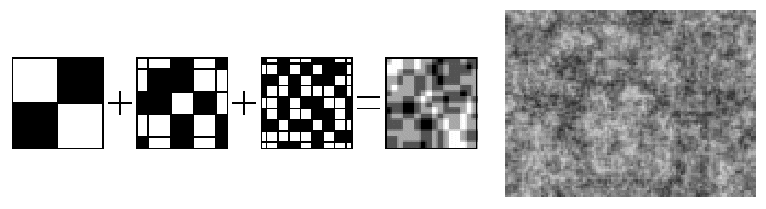
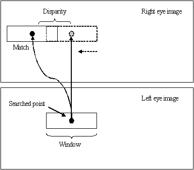
The matching is done by calculating a zero-mean normalized correlation criteria c(d) for a fixed size window with center at the point (x,y) of the rectified camera image with the same size window at the point (x+d,y) of the rectified pattern image.
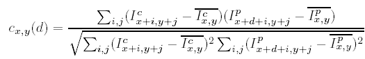
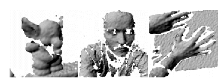
The 3D is reconstructed from the disparity map. Below are the examples of the reconstructions of three scenes made with this method. The scenes (from left to right) are an elephant toy, a face and hands.
Example of a Passive Stereoscopy Method
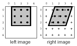
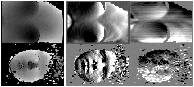
The passive stereoscopy method described in [4] proposes an enhanced correlation calculation mechanism. The technique involves calculation of the differential properties of the underlying scene surfaces directly from the stereoscopic images. The intensities of the pixels of a region of the left image are interpolated according to a hypothesis of the surface shape and how the surface of this shape would look on the right image (see picture from [4] below). The best match for a particular region of the left image is found for both the value of disparity and the values of the derivatives of the disparity over y and x using standard optimization methods.
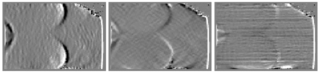
The properties of the underlying surfaces of the 3D scene are calculated from the map of the disparity and its first and second order derivatives. The examples (from [4]) of the results of using this method for textured 512x512 images of a human face and a bust:
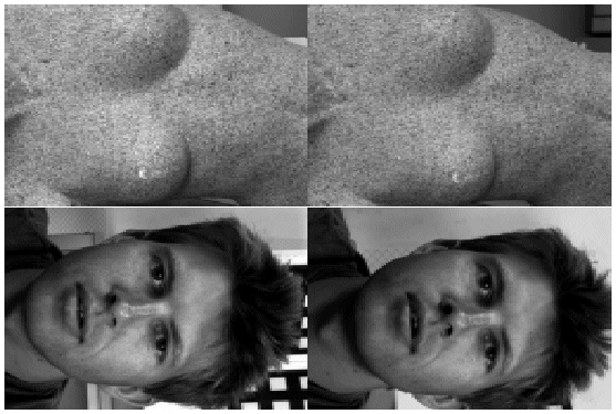
The original images (above), the disparity map, and its first derivatives (below).
The second derivatives of the disparity (below).
The face reconstruction (below)
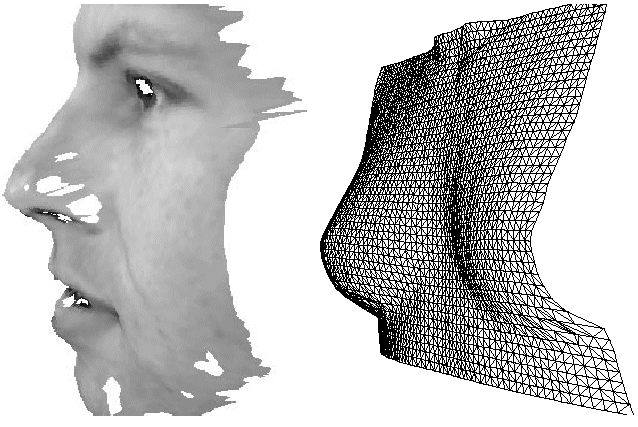
The disadvantage of this method is the extremely high computational cost.
Cooperation Of Edge Detection And Stereoscopy
Edge Detection Guided by Stereoscopy
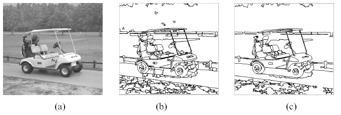
The most difficult problem of the edge detection is choosing a scale and edge acceptance thresholds to provide the best noise to data ratio. The work described in [3] proposes changing the scale of smoothing depending on the distance to the objects of the scene. The goal here is to be able to identify a military ordnance with equal possibility on different distances, which means preserving smaller details for greater distances. The examples from [3] are below.
The original image.
The disparity map of the image (below).
The edges detected with scale 1,2,4 and guided by stereoscopy (from left to right).
Approach
The results the stereoscopy shows on the real world scenes are far from being perfect. One of the problems here is the lack of the texture for matching areas of the stereoscopy pictures. The other problem is occlusions.
The traditional correlation calculation lays in the foundation of almost all stereoscopy techniques. Usually a rectangular window is placed around a point in question on one image and the correlation is calculated for the correspondent rectangular area in all the possible correspondent positions on the other image. The position of the point with the best matching correlation is then used to calculate the disparity.
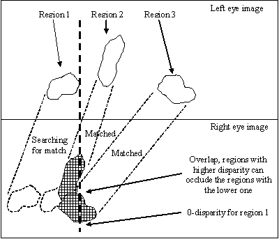
The approach proposed should (to some degree) eliminate the holes in the disparity map, improve the matching results by guaranteeing presence of a texture in the matching area, improve the performance by applying the disparity calculation to clusters of pixels and improve the matching quality by predicting and taking into account the occlusions while searching for a match.
The basic ideas are:
calculate the disparity for regions of an image;
use the image segmentation techniques to separate the image into a set of regions (assuming the regions represent the scene objects and/or their portions) for matching;
use the image the regions have come from to determine the correlation threshold to reject the false matches;
when matching a region, do not use pixels from the parts of the region occluded by the other regions that are closer to the cameras and are generating an acceptable match.
Algorithm
The algorithm takes two image files on input. The first file is a stereoscopic image of a scene comprised of the left eye picture followed by the right eye picture (see examples below). The second file is a segmented image of the left eye picture. The file is used to read a region map. Any image segmentation software producing a bitmap of regions where the adjacent regions are of unique uniform colors can be used to generate the second image.
The algorithm also takes a parameter, the minimum region overlap value, defining the minimum percentage of the pixels of the region that have to be used for the correlation calculation in order for the results of the calculation to be acceptable.
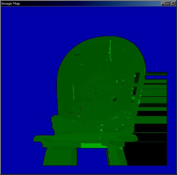
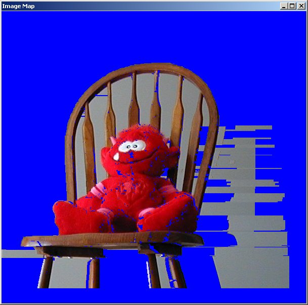
The output of the algorithm is an image representing the disparity map. The higher intensity of the green color means higher disparity values. The blue color maps the unmatched areas. The algorithm also can produce a target reconstruction map, which is the pixels of the left eye picture moved according to the disparity map to the shifted positions. Ideally the target reconstruction map should be a copy of the right eye picture.
The steps of the algorithm are outlined below:
Read the RGB values of the pixels of the left and the right eye pictures into the corresponded image objects;
Parse the region map image, initialize and add to a region list all (N) regions, fill in the left eye image region map with the region ids at the positions of the pixels of the regions, clean up the right eye region map;
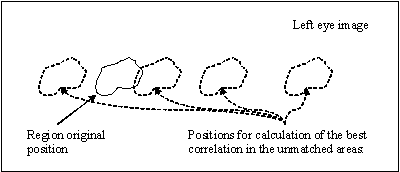
Calculate the best correlation in the unmatched areas (the value is calculated using the left eye image to estimate the correlation calculation results in the not matching areas of the right eye picture) for all the regions;
For all the regions not marked as done find their best matches on the right eye picture; use only the pixels of the right eye picture that yet have no region marked as done mapped to them;
The regions that cannot be matched on the right eye image using at least the minimum region overlap percentage of their pixels (because the disparity shifts them out or too many pixel positions on the right eye picture are already mapped to the other regions) are marked as no-match;
Compare the correlation calculated for the each successfully matched at the previous step region to the best correlation seen up to this point for the region and update the region's disparity and the correlation with the new values if the new correlation is better than the previously calculated ones;
Mark the region with the highest disparity (the closest to the cameras) and the correlation higher than the best correlation in the unmatched areas (calculated for the region at the step (3)) as done, fill in the right eye image region map with the region id in the adjusted to the disparity and yet clear positions (i.e. map the match);
Repeat the step (7) for all the regions that cannot overlap if moved horizontally.
If there has been no new regions marked as done at the previous two steps build the disparity map from the disparity calculated for the regions that are done and exit, otherwise return to the step (4);
The pictorial representation of several steps of the algorithm is presented below.
The step 2, - calculation of the best correlation in the unmatched areas:
The step 4, - search for the best match for a region of the left eye image on the right eye image:
Examples of current work
The developed code does not fully implement the algorithm yet. The code has evolved through several stages and the pictures presented below represent the major ones.
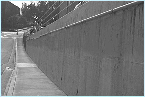
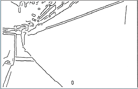
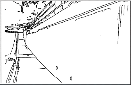
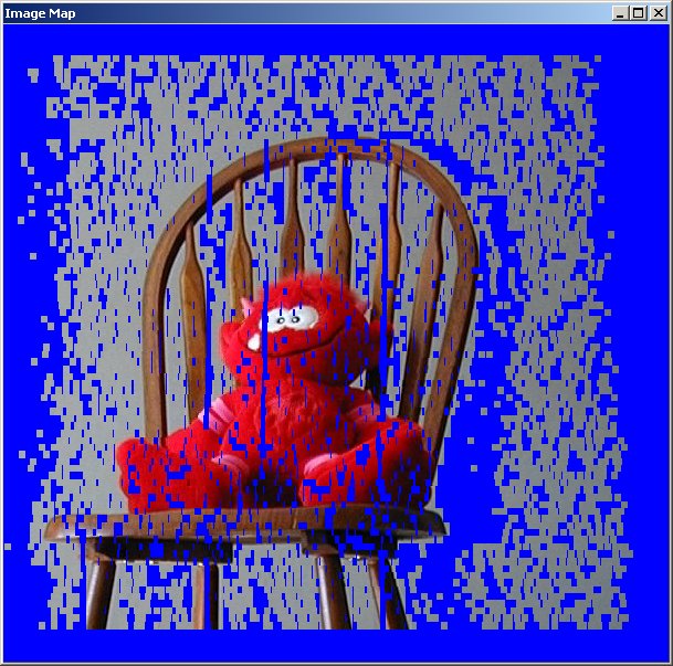
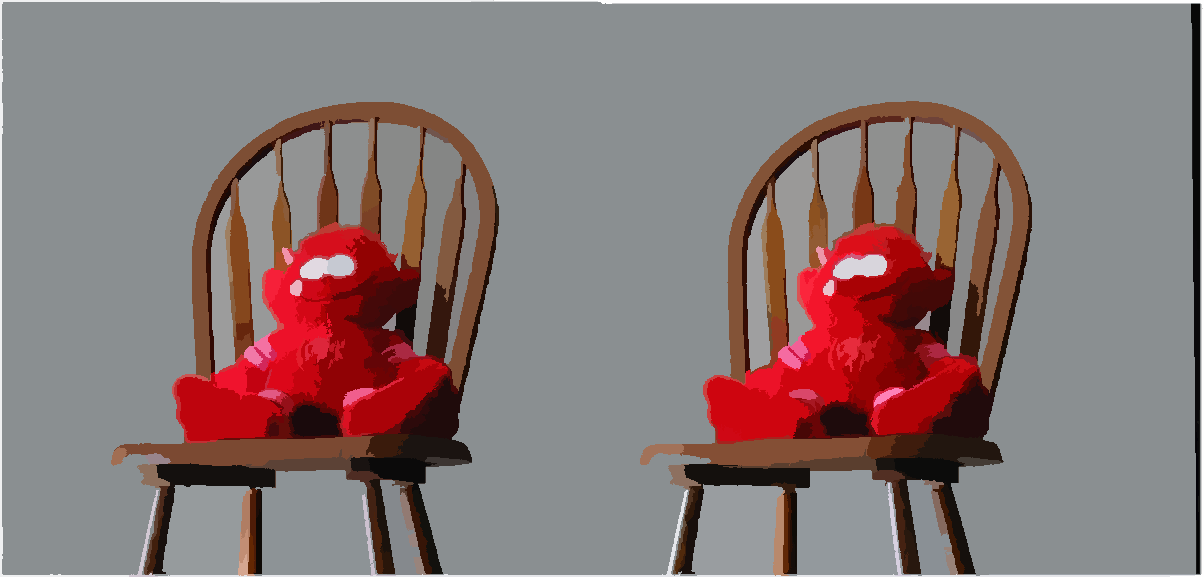
The source stereoscopic image:

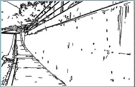
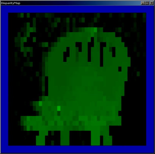
The initial implementation was doing simple square region fitting, the disparity was calculated for the square regions without accounting for the occlusions (the target map reconstruction was not implemented at the time).
The second version of the
code was still using square regions but it used the overlapping control in the
sense that it was more like building a mosaic from the tiles made of the left
image, although the tiles were allowed to overlap a little bit. The disparity map (for the
left eye view) and the target (right eye view) image reconstruction calculated
using the best square region fitting with overlap avoidance are below.
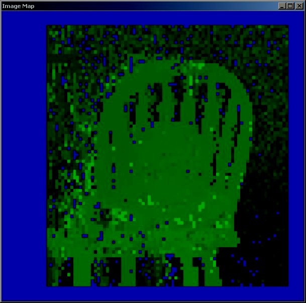
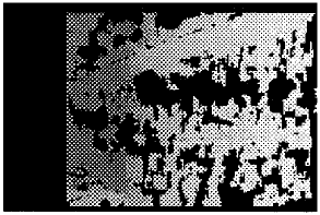
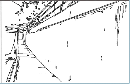
The third version used the image segmentation. The segmented image was build using the package EDISON (Edge Detection and Image Segmentation) described in [2]. The disparity map (for the left eye view), the target (right eye view) image reconstruction calculated using the best segmented region fitting with overlap avoidance, and the segment map used for the calculation are below.
The quality of the disparity map generated by the current code is too low to be used for the edge detection at the scale of the source image. Further improvements or the use of an image of a significantly higher resolution are required for producing better results. The use of the image segmentation for defining the search regions is surely beneficial since preserving the fine details of the scene objects, but it should be especially tuned for eliminating creation of huge regions that can suffer significant distortion and be hard to match. The application of the technique described in [4] can also be helpful when matching regions. All in all, further work is required to improve the stereoscopy quality on the real life scenes to the degree that it can be reliably used for the detection of the geometric properties of the scene objects.
Dejemel Ziou, Salvatore Tabbone. "EDGE DETECTION TECHNIQUES – AN OVERVIEW" (1997)
Christopher M. Christoudias, Bogdan Georgescu and Peter Meer. "SYNERGISM IN LOW LEVEL VISION"
Clark F Olson. "IMAGE SMOOTHING AND EDGE DETECTION GUIDED BY STEREOSCOPY" (1999)
Fre´de´ric Devernay, Olivier Faugeras. "COMPUTING DIFFERENTIAL PROPERTIES OF 3-D SHAPES FROM STEREOSCOPIC IMAGES WITHOUT 3-D MODELS" (1994)
Frédéric Devernay, Olivier Bantiche, Ève Coste-Manière, "STRUCTURED LIGHT ON DYNAMIC SCENES USING STANDARD STEREOSCOPY ALGORITHMS" (2002)
Ian L. Dryden, "Image Segmentation using Voronoi Polygons and MCMC, with Application to Muscle Fibre Images"
"Segmentation using the Watershed Transform" (http://www.mmorph.com/mmtutor1.0/html/mmtutor/mm080water.html)
Tu and S. C. Zhu, "Image Segmentation by Data-Driven Markov Chain Monte Carlo"